This article is mainly inspired by Jean-Philippe Vert's lecture on Kernel Methods.
Separable Case
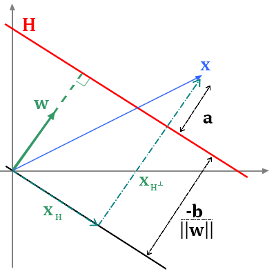
Let's work in dimension 2 ($x_1$ and $x_2$) and fix an hyperplane. The hyperplane is determined by is normal vector $w = (w_1,w_2)$ such that every point which
belong to this hyerplane verify the equation $w_1 x_1 + w_2 x_2 + b =0$.
Introduction
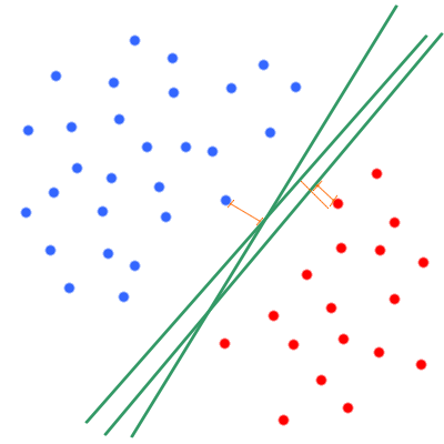
The Support Vector Machine (SVM) is a supervised machine learning technique to solve binary classification problems. The idea of SVM is to find the best hyperplane that will separate the data in two classes. The best hyperplane being defined by the one having the maximum margin for the most litigious point. For instance, let's visualize an example where the points are separable meaning that there exists an hyperplane (and more than one) thats separates the points perfectly into their orginal class.Linear SVM
Separable Case
Let's work in dimension 2 ($x_1$ and $x_2$) and fix an hyperplane. The hyperplane is determined by is normal vector $w = (w_1,w_2)$ such that every point which
belong to this hyerplane verify the equation $w_1 x_1 + w_2 x_2 + b =0$.
- $||w||=1$, we force the normal vector to be unitary. Any hyperplane can be defined by a unitary normal vector, nothing prevents us from doing that while we adjust the value of $b$
- Any hyperplane defined by $w$ and $b$ that verifies for a given $\alpha$ positif, that $\forall i = 1, \cdot, ... n, y_i(w^Tx_i+b) \geq \alpha$ is an hyperplane that perfectly separates the
points. Indeed, it means that every $x_i$ is on the right side of the hyperplane and at a distance from this hyperplane greater than $\alpha$. $\alpha$ is not necessarily the minimum margin,
in fact any value smaller or equal than the minimum margin works.
- And finally we take the max over all the possibilities, so we look for the hyperplane that separates the points and is as far as possible from all the points, so as far as possible from the
most litigious point
So the second equation does solve the same problem and we will focus on that one from now.
If we don't normalize $w$, we get a constraint of the for m $y_i(w^Tx_i+b) \geq \alpha ||w||$.
Thus, let's introduce $\alpha' = \alpha ||w||$, so problem gets
$$\underset{\alpha', w, b}{\max} \frac{\alpha'}{||w||} \text{ such that } y_i(w^Tx_i+b) \geq \alpha', \forall i = 1, \cdots, n$$
Let's rewrite once more the problem in its almost final form. The value of the margin $a$ is directly linked to the norm of $w$. If the norm increases, the coefficient $a$ decreases. So the problem
is the same if we fix $a=1$ and only "play" on the value of $w$. This lead us to the following equation:
$$\underset{w, b}{\max} \frac{1}{||w||} \text{ such that } y_i(w^Tx_i+b) \geq 1, \forall i = 1, \cdots, n$$
Though we don't have a quadratic programming problem which the king of problem we easily know how to solve. To get so, we say that maximizing over the inverse of $||w||$ is the same as minimizing
over $||w||$ and more specifically over $||w||^2$ which turn the problem quadratic. We add $\frac{1}{2}$ for computational convenience (the derivative will cancel the 2). We end up with a nice quadratic
programming problem: quadratic cost and linear constraints.
$$\underset{w, b}{\min} \frac{1}{2} ||w||^2 \text{ such that } y_i(w^Tx_i+b) \geq 1, \forall i = 1, \cdots, n$$
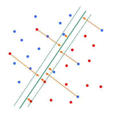
Non-Separable Case
Now the world is unfortunately not perfect, and the class are no longer linearly separable.
- if $y_i = 1$, $w^Tx_i + b \geq 1 - \xi_i$
- if $y_i = -1$, $w^Tx_i + b \leq -1 + \xi_i$
It summarizes in $y_i \left(w^Tx_i + b \geq 1 - \xi_i \right) \geq 1 - \xi_i$
- if $\xi_i = 0$, the point is far enough from the hyperplane and on the right side
- if $0<\xi_i \leq 1$, the point is on the right side, but it is litigious
- if $\xi_i>1$, an errors occurs
So $\sum_i \xi_i$ is an upper bound on the number of erros and we want this quantity to be as small as possible (in the separable case it worth 0). The optimisation problem becomes:
\begin{eqnarray}
& \underset{w, b}{\min} & \frac{1}{2} ||w||^2 + C \sum_i^n \xi_i \\
& \text{such that } & y_i(w^Tx_i+b) \geq 1 - \xi_i, \forall i = 1, \cdots, n \\
& & \xi_i \geq 0
\end{eqnarray}
The value of $C$ is arbitrary and must be choose by cross validation. Often SVM or referred as C-SVM, that is where the C comes from.
At optimum the slack variables worth either 0 or exactly 1 minus the distance from the hyperplane. So,
$$\xi_i = \max(0,1-y_i(w^Tx_i+b))$$
And just like this comes the final version of the problem !! The loss function $L$ to minimize is ...
\begin{eqnarray}
L(w) & = & \frac{1}{2} ||w||^2 + C \sum_i^n \max(0,1-y_i(w^Tx_i+b)) \\
& \propto & \sum_i^n \max(0,1-y_i(w^Tx_i+b)) + \lambda ||w||^2
\end{eqnarray}
With $\lambda = \frac{1}{C}$
Kernel SVM
In the linear case, the decision function $f$ is $f(x) = w^Tx_i + b$, so $L(w) = \sum_{i=1}^n \max(0,1-y_i f(x_i)) + \lambda ||w||^2$.
Let's introduce $\Phi_{hinge}(u) = \max(0,1-u)$, thus $L(w) = \sum_{i=1}^n \Phi(y_i f(x_i) + \lambda ||w||^2$.
This problem means that we are try to find a linear function $f$ that will minimize $f$. In order to kernelize the problem, we are now looking
for the function $f$ in the RKHS $\mathcal{H}$ defined by $K$ which minimize the new quantity:
$$L(f) = \frac{1}{n} \sum_{i=1}^n \Phi_{hinge}(y_i f(x_i)) + \lambda ||f||_{\mathcal{H}}$$
Remark: We can drop the 1/n, use $\lambda$ or $\lambda/2$ it doesn't change the problem.
Resolution
Let's recall the representer theorem.
- Let $\mathcal{X}$ be a set endowed with a positive definite kernel $K$, $\mathcal{H}_K$ the corresponding RKHS, and $S = \{x_1, \cdots, x_n \} \subset \mathcal{X}$
a finite set of point in $\mathcal{X}$.
- Let $\Psi: \mathbb{R}^{n+1} \rightarrow \mathbb{R}$ be a funtion of $n+1$ variables, stringly increasing with respect to the last variable.
- Then, any solution to the optimization problem:
$$\underset{f \in \mathcal{H}_K}{\min} \Psi(f(x_1),\cdots,f(x_n), ||f||_{\mathcal{H}_K})$$
admits a representation of the form:
$$\forall x \in \mathcal{X}, f(x) = \sum_{i=1}^n \alpha_i K(x_i,x)$$
How great this theorem is? Really great! First we learn that there is at least one solution. Second, even though the RKHS can be of infinite dimension, so that the solution
could be an infinite sum, we learn that it a finite sum and moreover a linear combination of the Kernel take over the training points!
If you don't know about kernel, you can found the results of linear SVM by replacing $K(x_i,x_j)$ by the scalar product that is $x_i^Tx_j$. This correspond to the linear Kernel.
We can thus apply the representer theorem to our problem because our problem fullfill all the conditions of the theorem.
Method 1
Let's note $K$ the matrix such that $[K]_{i,j} = K(x_i,x_j)$.
Thus $||f||_{\mathcal{H}} = \alpha^T K \alpha$, and the problems rewrites :
$$L = \frac{1}{n} \sum_{i=1}^n \Phi_{hinge}(y_i K \alpha) + \lambda \alpha^T K \alpha$$
Let's note $R(u) = \frac{1}{n} \sum_{i=1}^n \Phi_{hinge}(u)$.
The Frenchel-Legendre transform of a function $f : \mathbb{R}^N \rightarrow \mathbb{R}$ is the function $f^* : \mathbb{R}^N \rightarrow R$ defined by
$$f^*(u) = \underset{x \in \mathbb{R}^N}{\sup} < x,u > - f(x)$$
So let's compute the Frenchel-Legendre transform $R^*$ of $R$ in terms of $\Phi_{hinge}^*$ :
\begin{eqnarray}
R^{*}(u) &=& \underset{x \in \mathbb{R}^n}{\text{sup}} < x,u >-R(x) \\
&=& \underset{x \in \mathbb{R}^n}{\text{sup}} \sum_{i=1}^n x_i u_i -\frac{1}{n}\sum_{i=1}^n \Phi_{hinge}(x_i) \\
&=& \underset{x \in \mathbb{R}^n}{\text{sup}} \frac{1}{n} \sum_{i=1}^n n x_i u_i - \Phi_{hinge}(x_i) \\
&=& \underset{x \in \mathbb{R}^n}{\text{sup}} \frac{1}{n} \sum_{i=1}^n x_i (n u_i) - \Phi_{hinge}(x_i)\\
& \leq & \frac{1}{n} \sum_{i=1}^n \underset{x_i \in \mathbb{R}}{\text{sup}} (x_i (n u_i) - \Phi_{hinge}(x_i) \\
& \leq & \frac{1}{n} \sum_{i=1}^n \Phi_{hinge}^*(n u_i) \\
\end{eqnarray}
Though, the problem being at separated variables, we actually have $R^{*}(u) = \frac{1}{n} \sum_{i=1}^n \Phi_{hinge}^*(n u_i)$
Adding the slack variable $u = Y K \alpha$, where $Y$ is the diagonal matrix with entries $Y_{i,i} = y_i$, the problem can be rewritten as a constrained optimization problem
$$\underset{\alpha \in \mathbb{R}^n, u \in \mathbb{R}^n}{R(u)} + \lambda \alpha^T K \alpha \ \text{such that} \ u = Y K \alpha $$
There exist a constant $\mu \in \mathbb{R}^n$ such that the dual problem is written :
\begin{eqnarray*}
\underset{\mu \in \mathbb{R}^n}{\sup} \ \underset{\alpha \in \mathbb{R}^n,u \in \mathbb{R}^n}{\min} R(u) + \lambda \alpha^T K \alpha + \mu^T (u - Y K \alpha) &=&
\underset{\mu \in \mathbb{R}^n}{\sup} \left( \underset{\alpha \in \mathbb{R}^n}{\min} \lambda \alpha^T K \alpha -\mu^T Y K \alpha - \underset{u \in \mathbb{R}^n}{\sup} \left(- R(u) - \mu^T u \right) \right) \\
&=& \underset{\mu \in \mathbb{R}^n}{\sup} \left( \underset{\alpha \in \mathbb{R}^n}{\min} \lambda \alpha^T K \alpha -\mu^T Y K \alpha -R^{*}(-\mu) \right) \\
\end{eqnarray*}
We then note $g_{\mu}{\alpha} = \lambda \alpha^T K \alpha - \mu^T Y K \alpha$.
Thus $\nabla_{\alpha}g_{\mu} = 2 \lambda K \alpha - Y K \mu = K(2 \lambda - Y \mu)$. The problem being convexe, there exist a minimum $\alpha^*$ which can be found when the gradient is null, thus :
$$ \alpha^* = \frac{Y \mu}{2 \lambda} + \varepsilon$$
with $K \varepsilon = 0$
The dual problem is finally :
\begin{eqnarray*}
\underset{\mu \in \mathbb{R}^n}{\sup} \left( - R^{*}(-\mu) + \lambda \alpha^{*T} K \alpha^{*} - \mu^T K \alpha^{*} \right) &=& \underset{\mu \in \mathbb{R}^n}{\sup} - R^{*}(-\mu) + \frac{1}{4 \lambda} \mu^T K \mu - \frac{1}{2 \lambda} \mu^T K \mu \\
&=& \underset{\mu \in \mathbb{R}^n}{\sup} - R^{*}(-\mu) - \frac{1}{4\lambda} \mu^T K \mu \\
&=& \underset{\mu \in \mathbb{R}^n}{\sup} - R^{*}(\mu) - \frac{1}{4\lambda} \mu^T K \mu \\
&=& - \underset{\mu \in \mathbb{R}^n}{\min} R^{*}(\mu) + \frac{1}{4\lambda} \mu^T K \mu \\
&=& - \underset{\mu \in \mathbb{R}^n}{\min} \frac{1}{n}\sum_{i=1}^n \Phi_{hinge,y_i}^* (n\mu_i) + \frac{1}{4\lambda} \mu^T K \mu
\end{eqnarray*}
One can now (quite) easily check that:
$$
\Phi_{hinge,y}^*(u) = \left \{
\begin{aligned}
& yu & \text{if} \ yu \in [-1,0] \\
& + \infty & \text{otherwise}
\end{aligned}
\right.
$$
The problem can be now written:
\begin{eqnarray*}
- \underset{\mu \in \mathbb{R}^n}{\min} \frac{1}{n}\sum_{i=1}^n \Phi_{hinge,y_i}^* (n\mu_i) + \frac{1}{4\lambda} \mu^T K \mu &=& -\underset{\mu \in \mathbb{R}^n}{\min} \frac{1}{n} \sum_{i=1}^n n \mu_i y_i + \frac{1}{4\lambda} \mu^T K \mu \\
& & \text{with } n \mu_i y_i \in [-1,0] \\
&=& - \underset{\mu \in \mathbb{R}^n}{\min} \sum_{i=1}^n \mu_i y_i + \frac{1}{4\lambda} \mu^T K \mu \\
& & \text{with } \mu_i y_i \in [-1/n,0] \\
\end{eqnarray*}
Let's note $\forall i, \nu_i = -\mu_i y_i$.
We get:
$$ - \underset{0 \leq \nu \leq 1/n}{\min} \sum_{i=1}^n -\nu_i + \frac{1}{4\lambda} \sum_{i=1}^n \sum_{j=1}^n y_iy_j\nu_i\nu_j K(x_i,x_j)$$
So finally:
$$ \underset{0 \leq \nu_i \leq 1/n,\forall i}{\max} \sum_{i=1}^n \nu_i - \frac{1}{4\lambda} \sum_{i=1}^n \sum_{j=1}^n y_iy_j\nu_i\nu_j K(x_i,x_j)$$
Method 2
The initial minimization problem is:
$$L(f) = \frac{1}{n} \sum_{i=1}^n \Phi_{hinge}(y_i f(x_i)) + \lambda ||f||_{\mathcal{H}}$$
The optimization problem is convex but not differentiable, so for this method we reformulate the problem with the slack variables:
\begin{eqnarray}
& \underset{f \in \mathcal{H}, \xi \in \mathbb{R}^n}{\min} & \frac{1}{n} \sum_i^n \xi_i + \lambda ||f||^2_{\mathcal{H}} \\
& \text{subject to} & \xi_i \geq \Phi_{hinge}(y_if(x_i))
\end{eqnarray}
Thanks to the representer theorem we know that $f(x) = \sum_{i=1}^n \alpha_i K(x_i,x)$.
<\br>
The problem can be rewritten as an optimization problem in $\alpha$ and $\xi$:
\begin{eqnarray}
& \underset{f \in \mathcal{H}, \xi \in \mathbb{R}^n}{\min} & \frac{1}{n} \sum_i^n \xi_i + \lambda \alpha^T K \alpha \\
& \text{subject to} & y_i \sum_{i=1}^n \alpha_j K(x_i,x_j) + \xi_i -1 \geq 0 \\
& & \xi_i \geq 0
\end{eqnarray}
Let us then introduce the Lagrange multipliers $\mu \in \mathbb{R}^n$ and $\nu \in \mathbb{R}^n$. The Lagrangian problem is :
$$L(\alpha,\xi,\mu,\nu) = \frac{1}{n} \sum_i^n \xi_i + \lambda \alpha^T K \alpha - \sum_{i=1}^n \nu_i \left[y_i \sum_{j=1}^n \alpha_j K(x_i,x_j)+\xi-1 \right]
- \sum_{i=1}^n \mu_i \xi_i$$
Minimizing with respect to $\alpha$
$$\nabla_{\alpha} L = 2 \lambda K \alpha - K Y \nu = K(2 \lambda \alpha - Y \nu)$$
where $Y$ is the diagonal matrix with entries $Y_{i,i} = y_i$.
Solving $\nabla_{\alpha} L = 0$ leads do
$$ \alpha = \frac{Y \nu}{2\lambda} + \varepsilon$$
with $K \varepsilon = 0$, but $\varepsilon$ does not change $f$ so we can choose $\varepsilon = 0$.
Minimizing with respect to $\xi$
$L$ is a linear function in $\xi$ so its minimum is $- \infty$ except when $\nabla_{\xi} L = 0$, that is :
$$\frac{\partial L}{\partial \xi_i} = \frac{1}{n}-\mu_i-\nu_i = 0$$
We therefore obtain the Lagrange dual function:
\begin{eqnarray}
q(\mu,\nu) & = & \underset{\alpha \in \mathbb{R}^n, \xi \in \mathbb{R}^n}{\inf} L(\alpha,\xi,\mu,\nu) \\
& =& \left \{
\begin{aligned}
& \sum_{i=1}^n \nu_i - \frac{1}{4\lambda} \sum_{i=1}^n \sum_{j=1}^n y_iy_j\nu_i\nu_j K(x_i,x_j) & \text{if} \ \nu_i+\mu_i = \frac{1}{n} \forall i \\
& - \infty & \text{otherwise}
\end{aligned}
\right.
\end{eqnarray}
Finally, the dual problem is
\begin{eqnarray}
& \text{maximize} & q(\mu,\nu) \\
& \text{subject to} & \mu \geq 0, \nu \geq 0
\end{eqnarray}
Which is (hopefully) exactly the same problem as obtain with the first method ! Indeed,
- If $\nu_i \geq 1/n$ for some $i$, then $q(\mu,\nu) = - \infty$
- If $0 \leq \nu_i \leq 1/n$ for all $i$, then the dual function takes finite values that depend only on $\nu$ by taking $\mu_i = 1/n - \nu_i$
Why is it called Support Vector Machine ?
Solution
Once the dual problem is solved in $\nu$ we get a solution of the primal problem by $\alpha = \frac{Y\nu}{2 \lambda}$. We can
therefore directly plug this into the dual problem to obtain the QP that $\alpha$ must solve:
\begin{eqnarray}
& \underset{\alpha \in \mathbb{R}^d}{\max} & 2 \sum_i^n \alpha_i y_i - \sum_{i=1}^n \sum_{j=1}^n \alpha_i \alpha_j K(x_i,x_j) =
2 \alpha^T y - \alpha^T K \alpha \\
& \text{subject to} & 0 \leq \alpha_i y_i \leq \frac{1}{2 \lambda n}, \forall i
\end{eqnarray}
We apply the Karush-Kuhn-Tucker (KKT) theorem. The obtained conditions are:
- $\alpha_i \left[ y_i f(x_i) + \xi_1 -1 \right] = 0$
- $\left( \alpha_i - \frac{y_i}{2 \lambda n} \right) \xi_i = 0$
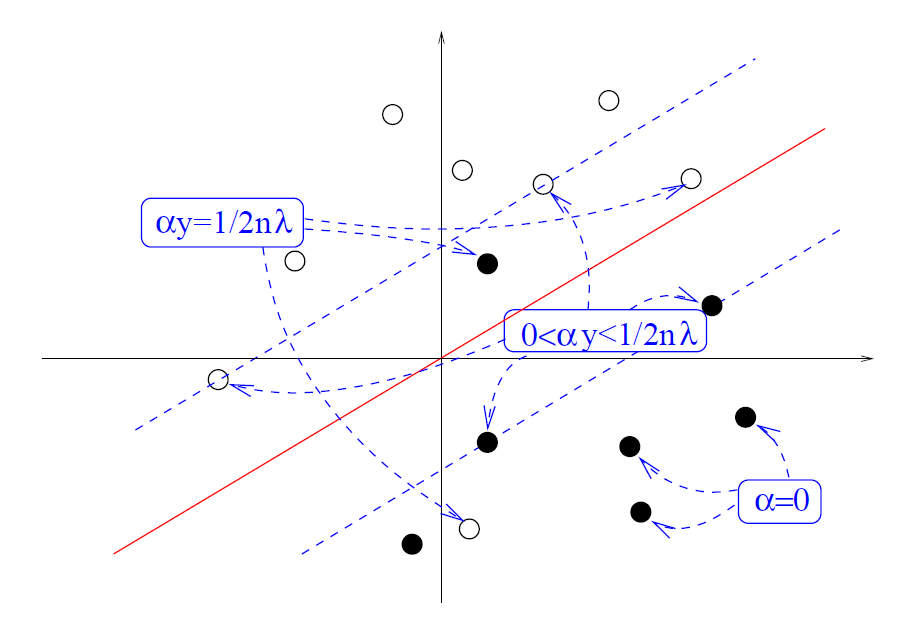
Three possibilities arises:
- If $\alpha_i = 0$, then the second constraint is active: $\xi_i=0$. This implies $y_i f(x_i) \geq 1$
- If $0 < y_i \alpha_i < \frac{1}{2 \lambda n}$, then both constraints are active: $\xi_i = 0$ and $y_i f(x_i) + \xi_i -1=0$.
This implies y_i f(x_i) = 1
- If $\alpha_i = \frac{y_i}{2 \lambda n}$, then the second constraint is not active ($\xi \geq 0$), while the first one is active:
$y_if (x_i)+\xi_i = 1$. Thus, $y_i f(x_i) \leq 1$
Vizualisation
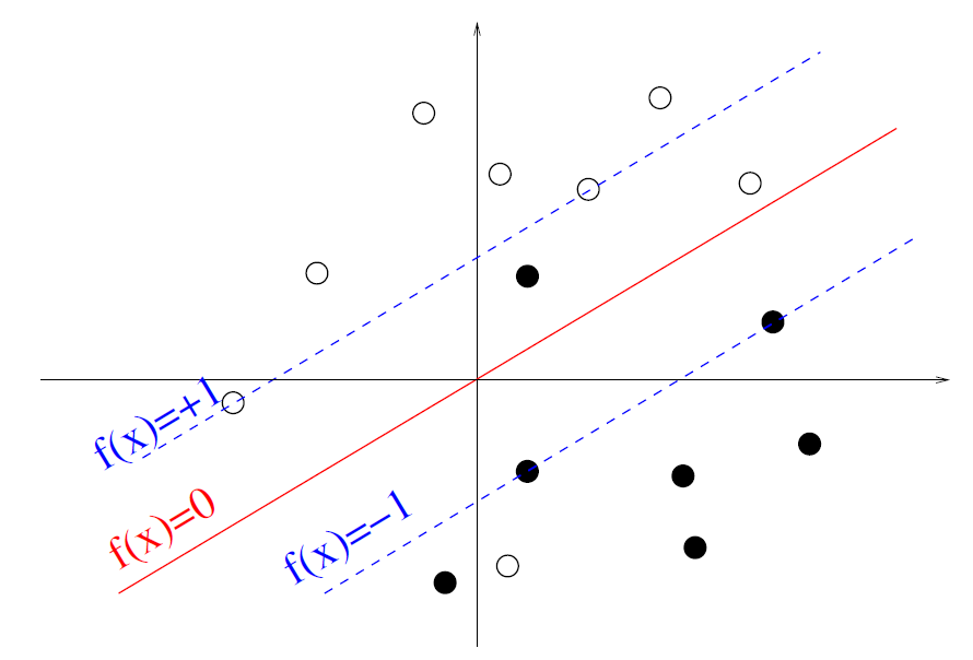
The support vector
Consequently to KKT conditions, many $\alpha_i$ worth 0. Thus, only the remaining training points with $\alpha_i \neq 0$ are involved in the computation of $f$.
They are called the support vectors.
$$\forall x, f(x) = \sum_{i=1}^n \alpha_i K(x_i,x) = \sum_{i \in SV} \alpha_i K(x_i,x)$$
with SV the set of support vectors.
This lead to sparse solution in $\alpha$ thus fast algorithms both for training and for classification of new points, since the evaluation has to be done only for
support vectors.
- if $y_i = 1$, $w^Tx_i + b \geq 1 - \xi_i$
- if $y_i = -1$, $w^Tx_i + b \leq -1 + \xi_i$
- if $\xi_i = 0$, the point is far enough from the hyperplane and on the right side
- if $0<\xi_i \leq 1$, the point is on the right side, but it is litigious
- if $\xi_i>1$, an errors occurs
Kernel SVM
In the linear case, the decision function $f$ is $f(x) = w^Tx_i + b$, so $L(w) = \sum_{i=1}^n \max(0,1-y_i f(x_i)) + \lambda ||w||^2$. Let's introduce $\Phi_{hinge}(u) = \max(0,1-u)$, thus $L(w) = \sum_{i=1}^n \Phi(y_i f(x_i) + \lambda ||w||^2$. This problem means that we are try to find a linear function $f$ that will minimize $f$. In order to kernelize the problem, we are now looking for the function $f$ in the RKHS $\mathcal{H}$ defined by $K$ which minimize the new quantity: $$L(f) = \frac{1}{n} \sum_{i=1}^n \Phi_{hinge}(y_i f(x_i)) + \lambda ||f||_{\mathcal{H}}$$ Remark: We can drop the 1/n, use $\lambda$ or $\lambda/2$ it doesn't change the problem.Resolution
Let's recall the representer theorem.- Let $\mathcal{X}$ be a set endowed with a positive definite kernel $K$, $\mathcal{H}_K$ the corresponding RKHS, and $S = \{x_1, \cdots, x_n \} \subset \mathcal{X}$ a finite set of point in $\mathcal{X}$.
- Let $\Psi: \mathbb{R}^{n+1} \rightarrow \mathbb{R}$ be a funtion of $n+1$ variables, stringly increasing with respect to the last variable.
- Then, any solution to the optimization problem: $$\underset{f \in \mathcal{H}_K}{\min} \Psi(f(x_1),\cdots,f(x_n), ||f||_{\mathcal{H}_K})$$ admits a representation of the form: $$\forall x \in \mathcal{X}, f(x) = \sum_{i=1}^n \alpha_i K(x_i,x)$$
Method 1
Let's note $K$ the matrix such that $[K]_{i,j} = K(x_i,x_j)$. Thus $||f||_{\mathcal{H}} = \alpha^T K \alpha$, and the problems rewrites : $$L = \frac{1}{n} \sum_{i=1}^n \Phi_{hinge}(y_i K \alpha) + \lambda \alpha^T K \alpha$$ Let's note $R(u) = \frac{1}{n} \sum_{i=1}^n \Phi_{hinge}(u)$. The Frenchel-Legendre transform of a function $f : \mathbb{R}^N \rightarrow \mathbb{R}$ is the function $f^* : \mathbb{R}^N \rightarrow R$ defined by $$f^*(u) = \underset{x \in \mathbb{R}^N}{\sup} < x,u > - f(x)$$ So let's compute the Frenchel-Legendre transform $R^*$ of $R$ in terms of $\Phi_{hinge}^*$ : \begin{eqnarray} R^{*}(u) &=& \underset{x \in \mathbb{R}^n}{\text{sup}} < x,u >-R(x) \\ &=& \underset{x \in \mathbb{R}^n}{\text{sup}} \sum_{i=1}^n x_i u_i -\frac{1}{n}\sum_{i=1}^n \Phi_{hinge}(x_i) \\ &=& \underset{x \in \mathbb{R}^n}{\text{sup}} \frac{1}{n} \sum_{i=1}^n n x_i u_i - \Phi_{hinge}(x_i) \\ &=& \underset{x \in \mathbb{R}^n}{\text{sup}} \frac{1}{n} \sum_{i=1}^n x_i (n u_i) - \Phi_{hinge}(x_i)\\ & \leq & \frac{1}{n} \sum_{i=1}^n \underset{x_i \in \mathbb{R}}{\text{sup}} (x_i (n u_i) - \Phi_{hinge}(x_i) \\ & \leq & \frac{1}{n} \sum_{i=1}^n \Phi_{hinge}^*(n u_i) \\ \end{eqnarray} Though, the problem being at separated variables, we actually have $R^{*}(u) = \frac{1}{n} \sum_{i=1}^n \Phi_{hinge}^*(n u_i)$ Adding the slack variable $u = Y K \alpha$, where $Y$ is the diagonal matrix with entries $Y_{i,i} = y_i$, the problem can be rewritten as a constrained optimization problem $$\underset{\alpha \in \mathbb{R}^n, u \in \mathbb{R}^n}{R(u)} + \lambda \alpha^T K \alpha \ \text{such that} \ u = Y K \alpha $$ There exist a constant $\mu \in \mathbb{R}^n$ such that the dual problem is written : \begin{eqnarray*} \underset{\mu \in \mathbb{R}^n}{\sup} \ \underset{\alpha \in \mathbb{R}^n,u \in \mathbb{R}^n}{\min} R(u) + \lambda \alpha^T K \alpha + \mu^T (u - Y K \alpha) &=& \underset{\mu \in \mathbb{R}^n}{\sup} \left( \underset{\alpha \in \mathbb{R}^n}{\min} \lambda \alpha^T K \alpha -\mu^T Y K \alpha - \underset{u \in \mathbb{R}^n}{\sup} \left(- R(u) - \mu^T u \right) \right) \\ &=& \underset{\mu \in \mathbb{R}^n}{\sup} \left( \underset{\alpha \in \mathbb{R}^n}{\min} \lambda \alpha^T K \alpha -\mu^T Y K \alpha -R^{*}(-\mu) \right) \\ \end{eqnarray*} We then note $g_{\mu}{\alpha} = \lambda \alpha^T K \alpha - \mu^T Y K \alpha$. Thus $\nabla_{\alpha}g_{\mu} = 2 \lambda K \alpha - Y K \mu = K(2 \lambda - Y \mu)$. The problem being convexe, there exist a minimum $\alpha^*$ which can be found when the gradient is null, thus : $$ \alpha^* = \frac{Y \mu}{2 \lambda} + \varepsilon$$ with $K \varepsilon = 0$ The dual problem is finally : \begin{eqnarray*} \underset{\mu \in \mathbb{R}^n}{\sup} \left( - R^{*}(-\mu) + \lambda \alpha^{*T} K \alpha^{*} - \mu^T K \alpha^{*} \right) &=& \underset{\mu \in \mathbb{R}^n}{\sup} - R^{*}(-\mu) + \frac{1}{4 \lambda} \mu^T K \mu - \frac{1}{2 \lambda} \mu^T K \mu \\ &=& \underset{\mu \in \mathbb{R}^n}{\sup} - R^{*}(-\mu) - \frac{1}{4\lambda} \mu^T K \mu \\ &=& \underset{\mu \in \mathbb{R}^n}{\sup} - R^{*}(\mu) - \frac{1}{4\lambda} \mu^T K \mu \\ &=& - \underset{\mu \in \mathbb{R}^n}{\min} R^{*}(\mu) + \frac{1}{4\lambda} \mu^T K \mu \\ &=& - \underset{\mu \in \mathbb{R}^n}{\min} \frac{1}{n}\sum_{i=1}^n \Phi_{hinge,y_i}^* (n\mu_i) + \frac{1}{4\lambda} \mu^T K \mu \end{eqnarray*} One can now (quite) easily check that: $$ \Phi_{hinge,y}^*(u) = \left \{ \begin{aligned} & yu & \text{if} \ yu \in [-1,0] \\ & + \infty & \text{otherwise} \end{aligned} \right. $$ The problem can be now written: \begin{eqnarray*} - \underset{\mu \in \mathbb{R}^n}{\min} \frac{1}{n}\sum_{i=1}^n \Phi_{hinge,y_i}^* (n\mu_i) + \frac{1}{4\lambda} \mu^T K \mu &=& -\underset{\mu \in \mathbb{R}^n}{\min} \frac{1}{n} \sum_{i=1}^n n \mu_i y_i + \frac{1}{4\lambda} \mu^T K \mu \\ & & \text{with } n \mu_i y_i \in [-1,0] \\ &=& - \underset{\mu \in \mathbb{R}^n}{\min} \sum_{i=1}^n \mu_i y_i + \frac{1}{4\lambda} \mu^T K \mu \\ & & \text{with } \mu_i y_i \in [-1/n,0] \\ \end{eqnarray*} Let's note $\forall i, \nu_i = -\mu_i y_i$. We get: $$ - \underset{0 \leq \nu \leq 1/n}{\min} \sum_{i=1}^n -\nu_i + \frac{1}{4\lambda} \sum_{i=1}^n \sum_{j=1}^n y_iy_j\nu_i\nu_j K(x_i,x_j)$$ So finally: $$ \underset{0 \leq \nu_i \leq 1/n,\forall i}{\max} \sum_{i=1}^n \nu_i - \frac{1}{4\lambda} \sum_{i=1}^n \sum_{j=1}^n y_iy_j\nu_i\nu_j K(x_i,x_j)$$Method 2
The initial minimization problem is: $$L(f) = \frac{1}{n} \sum_{i=1}^n \Phi_{hinge}(y_i f(x_i)) + \lambda ||f||_{\mathcal{H}}$$ The optimization problem is convex but not differentiable, so for this method we reformulate the problem with the slack variables: \begin{eqnarray} & \underset{f \in \mathcal{H}, \xi \in \mathbb{R}^n}{\min} & \frac{1}{n} \sum_i^n \xi_i + \lambda ||f||^2_{\mathcal{H}} \\ & \text{subject to} & \xi_i \geq \Phi_{hinge}(y_if(x_i)) \end{eqnarray} Thanks to the representer theorem we know that $f(x) = \sum_{i=1}^n \alpha_i K(x_i,x)$. <\br> The problem can be rewritten as an optimization problem in $\alpha$ and $\xi$: \begin{eqnarray} & \underset{f \in \mathcal{H}, \xi \in \mathbb{R}^n}{\min} & \frac{1}{n} \sum_i^n \xi_i + \lambda \alpha^T K \alpha \\ & \text{subject to} & y_i \sum_{i=1}^n \alpha_j K(x_i,x_j) + \xi_i -1 \geq 0 \\ & & \xi_i \geq 0 \end{eqnarray} Let us then introduce the Lagrange multipliers $\mu \in \mathbb{R}^n$ and $\nu \in \mathbb{R}^n$. The Lagrangian problem is : $$L(\alpha,\xi,\mu,\nu) = \frac{1}{n} \sum_i^n \xi_i + \lambda \alpha^T K \alpha - \sum_{i=1}^n \nu_i \left[y_i \sum_{j=1}^n \alpha_j K(x_i,x_j)+\xi-1 \right] - \sum_{i=1}^n \mu_i \xi_i$$Minimizing with respect to $\alpha$
$$\nabla_{\alpha} L = 2 \lambda K \alpha - K Y \nu = K(2 \lambda \alpha - Y \nu)$$ where $Y$ is the diagonal matrix with entries $Y_{i,i} = y_i$. Solving $\nabla_{\alpha} L = 0$ leads do $$ \alpha = \frac{Y \nu}{2\lambda} + \varepsilon$$ with $K \varepsilon = 0$, but $\varepsilon$ does not change $f$ so we can choose $\varepsilon = 0$.Minimizing with respect to $\xi$
$L$ is a linear function in $\xi$ so its minimum is $- \infty$ except when $\nabla_{\xi} L = 0$, that is : $$\frac{\partial L}{\partial \xi_i} = \frac{1}{n}-\mu_i-\nu_i = 0$$ We therefore obtain the Lagrange dual function: \begin{eqnarray} q(\mu,\nu) & = & \underset{\alpha \in \mathbb{R}^n, \xi \in \mathbb{R}^n}{\inf} L(\alpha,\xi,\mu,\nu) \\ & =& \left \{ \begin{aligned} & \sum_{i=1}^n \nu_i - \frac{1}{4\lambda} \sum_{i=1}^n \sum_{j=1}^n y_iy_j\nu_i\nu_j K(x_i,x_j) & \text{if} \ \nu_i+\mu_i = \frac{1}{n} \forall i \\ & - \infty & \text{otherwise} \end{aligned} \right. \end{eqnarray} Finally, the dual problem is \begin{eqnarray} & \text{maximize} & q(\mu,\nu) \\ & \text{subject to} & \mu \geq 0, \nu \geq 0 \end{eqnarray} Which is (hopefully) exactly the same problem as obtain with the first method ! Indeed,- If $\nu_i \geq 1/n$ for some $i$, then $q(\mu,\nu) = - \infty$
- If $0 \leq \nu_i \leq 1/n$ for all $i$, then the dual function takes finite values that depend only on $\nu$ by taking $\mu_i = 1/n - \nu_i$
Why is it called Support Vector Machine ?
Solution
Once the dual problem is solved in $\nu$ we get a solution of the primal problem by $\alpha = \frac{Y\nu}{2 \lambda}$. We can therefore directly plug this into the dual problem to obtain the QP that $\alpha$ must solve: \begin{eqnarray} & \underset{\alpha \in \mathbb{R}^d}{\max} & 2 \sum_i^n \alpha_i y_i - \sum_{i=1}^n \sum_{j=1}^n \alpha_i \alpha_j K(x_i,x_j) = 2 \alpha^T y - \alpha^T K \alpha \\ & \text{subject to} & 0 \leq \alpha_i y_i \leq \frac{1}{2 \lambda n}, \forall i \end{eqnarray} We apply the Karush-Kuhn-Tucker (KKT) theorem. The obtained conditions are:- $\alpha_i \left[ y_i f(x_i) + \xi_1 -1 \right] = 0$
- $\left( \alpha_i - \frac{y_i}{2 \lambda n} \right) \xi_i = 0$
- If $\alpha_i = 0$, then the second constraint is active: $\xi_i=0$. This implies $y_i f(x_i) \geq 1$
- If $0 < y_i \alpha_i < \frac{1}{2 \lambda n}$, then both constraints are active: $\xi_i = 0$ and $y_i f(x_i) + \xi_i -1=0$. This implies y_i f(x_i) = 1
- If $\alpha_i = \frac{y_i}{2 \lambda n}$, then the second constraint is not active ($\xi \geq 0$), while the first one is active: $y_if (x_i)+\xi_i = 1$. Thus, $y_i f(x_i) \leq 1$
Vizualisation