Ridge and LASSO regressions are two common ways to regularized linear regression in order to avoid overfitting. LASSO has a tendency to
put some coefficient exactly equal to 0, which is almost never the case for Ridge regression. There is a theoretical explanation based on
the non differentiability of the absolute value on 0, but here we will focus on geometric interpretation which help to see clearer.
Let's formalize the problem in dimension 2. To objective of the linear regression is to find the coefficient $\beta_0$, $\beta_1$ and $\beta_2$ in order to
minimize $$f(\beta) = \sum_{i=1}^n (y_i - (\beta_1 x_{i,1} + \beta_2 x_{i,2} + \beta_0))^2$$.
Penalisation add constraint to this problem :
- Ridge : such that $||\beta_1||^2 + ||\beta_2||^2 < \mu$ which thanks to Lagrange multiplier reformulate the problem as
$\sum_{i=1}^n (y_i - (\beta_1 x_{i,1} + \beta_2 x_{i,2} + \beta_0))^2 + \lambda (||\beta_1||^2 + ||\beta_2||^2)$
- LASSO : such that $|\beta_1| + |\beta_2| < \mu$ which thanks to Lagrange multiplier reformulate the problem as
$\sum_{i=1}^n (y_i - (\beta_1 x_{i,1} + \beta_2 x_{i,2} + \beta_0))^2 + \lambda (|\beta_1| + |\beta_2|)$
We note $g_{Ridge}(\beta) = \lambda (||\beta_1||^2 + ||\beta_2||^2)$ and $g_{LASSO}(\beta) = \lambda (|\beta_1| + |\beta_2|)$.
The first term in the minimisation problem is $f(\beta)$ which is a conic. Let's compute what conic it is.
If we expand the formula, we get :
| $\sum_{i=1}^n (y_i - (\beta_1 x_{i,1} + \beta_2 x_{i,2} + \beta_0))^2$ |
$=\sum_{i=1}^n y_i^2 + (\beta_1 x_{i,1} + \beta_2 x_{i,2} + \beta_0)^2 - 2(\beta_1 x_{i,1} + \beta_2 x_{i,2} + \beta_0) y_i$
|
|
$=\sum_{i=1}^n y_i^2 + \beta_1^2 x_{i,1}^2 + \beta_2^2 x_{i,2}^2 + \beta_0^2 + 2 \beta_1 \beta_2 x_{i,2} x_{i,1} + 2 \beta_0 \beta_1 x_{i,1} + 2 \beta_0 \beta_2 x_{i,2}
- 2(\beta_1 x_{i,1} + \beta_2 x_{i,2} + \beta_0)y_i$ |
|
$=(\sum_{i=1}^n x_{i,1}^2) \beta_1^2 + (2 \sum_{i=1}^n x_{i,2} x_{i,1}) \beta_1 \beta_2 + (\sum_{i=1}^n x_{i,2}^2) \beta_2^2 + (2 \sum_{i=1}^n (\beta_0 - y_i) x_{i,1}) \beta_1
+ (2 \sum_{i=1}^n (\beta_0 - y_i) x_{i,2}) \beta_2 + (\sum_{i=1}^n \beta_0^2 - 2 \beta_0 y_i)$ |
|
$=A \beta_1^2 + B \beta_1 \beta_2 + C \beta_2^2 + D \beta_1 + E \beta_2 + F$ |
With,
| $A=$ | $\sum_{i=1}^n x_{i,1}^2$ |
| $B=$ | $2 \sum_{i=1}^n x_{i,2} x_{i,1}$ |
| $C=$ | $\sum_{i=1}^n x_{i,2}^2$ |
| $D=$ | $2 \sum_{i=1}^n (\beta_0 - y_i) x_{i,1}$ |
| $E=$ | $2 \sum_{i=1}^n (\beta_0 - y_i) x_{i,2}$ |
| $F=$ | $\sum_{i=1}^n \beta_0^2 - 2 \beta_0 y_i$ |
There are three possibilities (see
wikipedia)
- $B^2-4AC <0$, the equation represents an ellipse
- $B^2-4AC =0$, the equation represents a parabola
- $B^2-4AC >0$, the equation represents a hyperbola
Here we have, $B^2-4AC = 4 [(\sum_{i=1}^n x_{i,2} x_{i,1})^2 - \sum_{i=1}^n x_{i,1}^2 \sum_{i=1}^n x_{i,2}^2]$ which is negative thanks to
Cauchy–Schwarz inequality. Thus, we have an ellipse.
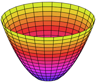
Although, we cannot always have $f(\beta) = 0$, we want to minimize $f$, so for a given value of $\beta$ we have $f(\beta) = m_{\beta}$. So the conic
equation changes to $F_{\beta} = F-m_{\beta}$, so in the 3D space $(\beta_1,\beta_2,z)$, we can a parabola where each cut by the plan $z=constant$ is an ellipse.
In the reduce form of the equation, the radius of the ellipse are proportional to $-F_{\beta} = m_{\beta}-F$, thus if $m_{\beta}$ increase, the radius increase.
Once projected on the plan $(\beta_1,\beta_2)$, we get an ellipse which a certain angle (which can be expressed from A,C and B), not necessary centered.
The representation of the penalty term is much more easy.
- $g_{Ridge}(\beta) = c_{\beta}^{Ridge}$ is a circle of radius $c_{\beta}^{Ridge}$
- $g_{LASSO}(\beta) = c_{\beta}^{LASSO}$ is a square of demi-diagonal $c_{\beta}^{LASSO}$
The aim is to minimize over a constraint, thus the two graphs have to meet otherwise the constraint is not fulfilled.
Let's say we have fix the size of the penalty (usually we test different value of the penalty through the choice of $\lambda$
and perform K-fold cross validation to select the best one). If the ellipse doesn't meet the penalty area, we have the increase
the size of the ellipse up to cross the penalty. The minimisation of the sum of the two terms hence is achieved on the edge of
the penalty area.