The aim of this post is to present some tools used by data scientist to solve their everyday life project, but not to give a theoretical lecture
about machine learning. This post is for non data scientist that want to know what data scientist does. You will discover what a data scientist has
to do, not how to do it.
Most of the knowledge of a data scientist is machine learning but most of this work consist in preprocessing data in order to have a clean input
table with the right variable for the model. The first part of this post will be about machine learning techniques and the second part about getting clean
data.
Machine learning
Supervised Learning
Presentation
The goal of supervised learning is to find a function $f$ that will explain the causality action between the input $X$ (for instance age of
a patient, sex, different medical measure) and the output $Y$. The output must take different form : is the patient sick or not (binary classification),
what is his disease (classification), what his white blood cell rate (regression).
This domain is call supervised learning, because we know what we have to predict. The data scientist have in his hand the inputs $X$ for different
patient, says $n$, with $p$ informations for each one, thus $X$ is a matrix with $n$ row and $p$ columns; and the corresponding output for each patient
$Y$ which his a vector of length $n$. The purpose is to find the best function $f$ such that $f(X)$ is close to $Y$, thereby, if a new patient comes and
we know the $p$ informations we need to know, by applying the function $f$ we get an estimation of the output for this person.
Loss function
What we are looking for is a function $f$ such that $f(X)$ is close to $Y$. But what does close mean mathematically speaking ? Is 3 close to 1 ? We have to define something
that will measure how far $f(X)$ (a vector of length $n$) is from $Y$ (an other vector of length $n$) : this new function $\ell$ is call the loss function.
The choice of $\ell$ is quite open as long as it as the mathematical properties of a distance.
However open, the choice of the loss function is very important and conditioned the best choice of $f$ si the best $f$ will be according to this particular choice
of the loss function. For different loss functions, the best $f$ is very likely to be different (we'll see example later). Here are different loss functions.
loss function
formula
comments
0/1 loss
$\ell(y,f(x)) = \sum_{i=1}^n 1(y_i f(x_i)<0) $
Only for problem where $y = \pm 1$. The error if $1$ is the sign of $f$ is different from
the sign of $y$ and $0$ otherwise
quadratic loss
$\ell(y,f(x)) = \sum_{i=1}^n ||y_i - f(x_i)||^2$
This will give much more weight to big error since the difference is up to
square
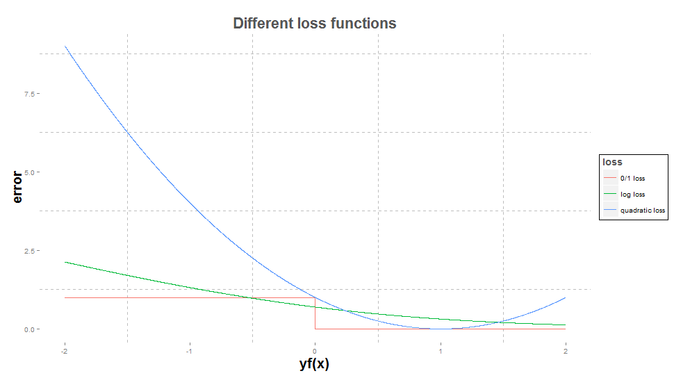
If $y=\pm1$, the quadratic loss can also be written $\ell(y,f(x)) = \sum_{i=1}^n ||1 - y_i f(x_i)||^2$. we can then plot this 3 loss functions with $yf(x)$ on the
horizontal axis and the error on the vertical axis.
Interpretation:
The 0/1 loss is very particular and make no distinction is whether you make a huge mistake or not. Moreover, a small variation of the output
can change completely the error. If the prediction is a small positive number, adding some noise can make the prediction a small negative number and the error would go from 0 to 1.
This loss function is not continuous.
The quadratic loss is minimum when when $y=f(x)$, is symmetric in 1 and increases really quickly as $f$ gets far from $y$. Saying $3$ to predict $1$ is as bad as saying $1$ to predict $-1$.
This can be argue because it one case we get the right sign ...
On the contrary, if $f$ and $y$ have the same sign, the higher $f$, the smaller the error. The idea is that if we said $100$ it means that we are really sure that the result is positive thus is $1$
The objective of supervised learning being to find the function $f$ closest to $Y$, i.e we want to find the function $f$ such that $\ell(Y,f(X))$ is minimum.
In maths, we note that :
$$\underset{f}{\arg \min} \quad \ell(Y,f(X))$$
for each function $f$ we get the value of $\ell(Y,f(X)$
we look for the minimum
we return the function $f$ for which we get the minimum (that's what "arg" means : we don't want the value of the minimum but the function that reaches this
minimum)
The only thing left to define is $f$. We are now facing an optimisation problem. This cannot be solved for any type of function for $f$ nor $\ell$, and the way
to find the solution also depends on the "form" of $f$ and $\ell$.
For instance,
$f$ can be linear : if the vector $x = (x_1,...,x_p)$, there exist a vector $a = (a_1,...,a_p)$ such that
$f(x) = a_1 x_1+ ... + a_p x_p = \sum_{i=1}^p a_i x_i$
$f$ can be a transformation of a linear product : $f(x) = \frac{1}{1+\exp(-\sum_{i=1}^p a_i x_i)}$
$f$ can be a polynomial in a degree $q$ higher than 1 (degree 1 = linear) : $f(x) = \sum_{i=1}^p a_i x_i^q$
$f$ can a combination of different functions. For instance, let's note $f_q(x)$ the function $\sum_{i=1}^p a_i x_i^q$. We
could have $f(x) = \sum_{q=1}^Q f_q(x)$
...
The choice of the loss function and the form of $f$ will defined the model. Let's give some example.
Does the choice of the loss function really matters?
Of course. Let's compare the error on the same data of two linear functions for the quadratic loss and the log loss.
For simplicity let's consider $n=2$ and $p=2$.
$$ X = \left( \begin{array}{cc}
2 & 4 \\
-3 & -0.5
\end{array} \right)
\text{ and }
Y = \left( \begin{array}{c}
1 \\ -1
\end{array} \right)
$$
Furthermore let's say we want to compare those two functions, $f_1(x) = 10x_1+4x_2$ and $f_2(x) = 0.2x_1+0.6x_2$.
Let's compute each error.
So according to quadratic loss, $f_2$ is $100$ times better than $f_1$ but according to the log loss, $f_1$ is $10^{14}$ times better than $f_2$ !!!!
So according to you, who's best ? $f_1$ says $36$ to predict $+1$ and $-32$ to predict $-1$ while $f_2$ says $2.8$ to predict $+1$ and $-0.9$ to predict $-1$.
If you want to say $f_2$ it's because I cheat a little. If you look at the previous table, when using the log loss, $f$ is not purely linear. $f$ is supposed to
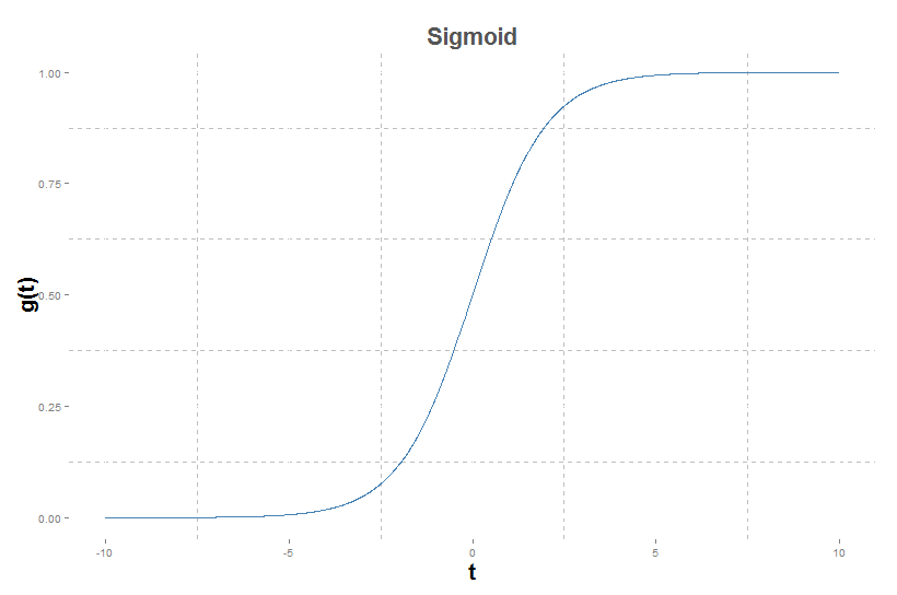
be a transformation of a linear regression. This transformation's role is to scale the function between 0 and 1. We then multiply this transformation by 2 and delete 1
to get something between -1 and 1. The first transformation name is called a sigmoid : $g(t) = \frac{1}{1+\exp(-t)}$
Thus the real $f_1$ and $f_2$ are :
$f_1(x) = \frac{2}{1+\exp(-(10x_1+4x_2))}-1$. The predicted values are then $1$ and $-1$.
$f_2(x) = \frac{2}{1+\exp(-(0.2x_1+0.6x_2))}-1$. The predicted values are then $0.88$ and $-0.42$.
That's the whole idea of logistic regression. The aim is to used a linear function and says "if you get something really positively (resp. negative) big we have a high
level of confidence in saying this is a 1 (resp. -1)". Then we use a little transformation to scale this number between -1 and 1. So saying $38$ to predict $1$ it's not
making a huge mistake but on the contrary being really sure the results is positive !
The best solution is then $f_1$.
Eventually, the choice of the loss function really matters and depends on the problem. If you want to predict a binary output, you'd better use the log loss.
Overfitting
Overfitting is one of the most important concept to know in machine learning in order to understand what makes a predictive model. The term explain
itself : overfitting is when one want to fit too much the training data. The real aim of machine learning is not to find the best function
to have the most little error on training data, but the one that will generalize best, i.e the one that will have the most little error when
new data will come. Remember that we want to make a prediction not just have a function that goes exactly through all our training point : that
is a interpolation problem and is no use for us.
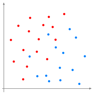
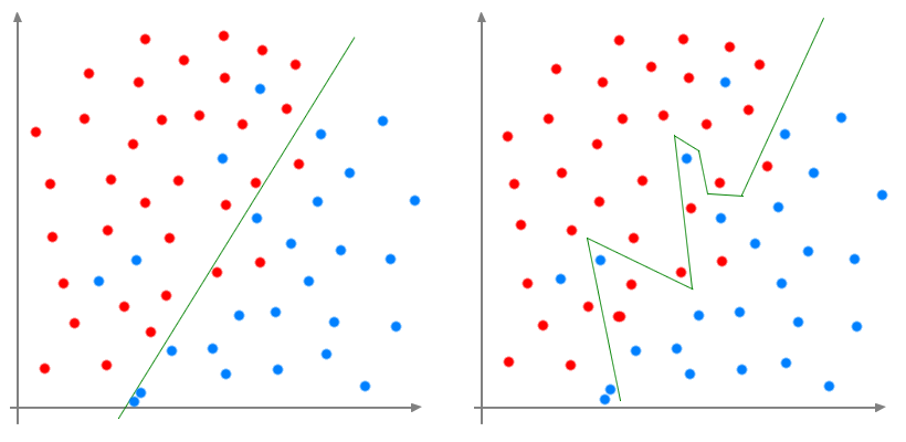
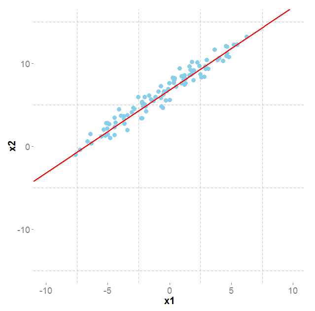
For instance let's imagine a binary classification problem. Some dots are blue other or red. We want to find a function that will cut the space in
order to have blue dots on one side of the function and red dots on the other side.
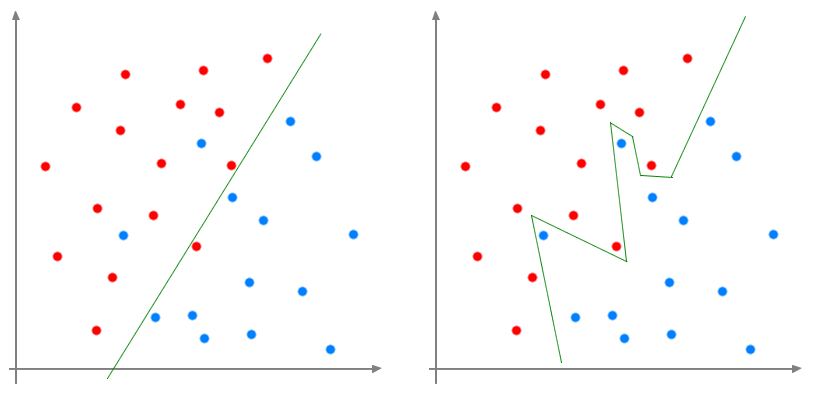
So we can draw a line which doesn't give a perfect separation but most of the red and blue points are at a different side of the lines. If we want a
model with a smaller training error, we should have a more complex line that will cut exactly the two groups.
Thus we will get a "perfect" model with
zero error. But the data we have a just a very tiny little fraction of the data that exist. If we want to predict if a patient has a disease or not,
we will have the observation for hundreds or thousands, but we want the model to predict the result for the other billions of humans being. So let's
add many new patients to the initial plot.
The complex line doesn't give perfect result any more! It is even worse that with just a classic line. The more points we add, the less precise the
complex model becomes, although the linear model keep a constant error. By complexifying too much the model, we learnt
nothing about the impact of the variables on the target, we just draw a line around points. On the contrary, the linear model learnt the impact. It's
not perfect for many reasons (maybe some explicative variables were missing and instead of 2 variables we needed 5, some interaction are still not
explain by human knowledge, some variable are not measurable like the will power of the patient, ...) but at least we were able to qualify the weight
of the variables at our disposal and have a model with a good generalization power.
The are two kinds of behaviours that can lead to overfitting :
Adding too many variables that have no explaining power. One should use statistics method to select the "good" variables
Choosing a too complex model
How to measure the performance ?
As seen in the last section, the aim is to have a model that will generalize well. But how can we know if a model will?
The most common method is called K-fold cross validation. The idea is to choose randomly 80% of the known data to estimate the
model, and apply the model on the 20% left. The selected data are called the training data, and the left ones or call the test data. We can that
apply the model on the test, which weren't use to train the model so doesn't bias the model to go in their own direction, and compare the result
with the real value since we got them. We repeat this process K times, usually 10 times, and compare the training errors to the test errors.
Obviously the test errors will be greater than the training errors but if the degradation is not too significant, we can have a strong confidence
on the generalization performance of the model.
Other models
Many other model exists. Let's just cite some if you want to know some names to shine in society or dig on the web : logistic regression,
ridge regression, LASSO regression, SVM, generalized linear model (GLM), trees, random forest, neural network, generative model, ...
Unsupervised Learning
Presentation
In unsupervised learning there is no explicit variable to predict, which is a huge advantage compared to supervised learning. While supervised learning
must wait label data or ask manual labelisation to create a training set, unsupervised learning can start immediately. Most of the time, unsupervised learning
is about clustering: the goal is to identify homogeneous group from the data in order to extract different behaviours. For instance one may want to identify user
behaviour on website. By gathering user interactions (click history, time of logging, number of purchase, time spend on the website, ...), we can then apply a clustering
algorithm to identify group of user with similar behaviour (window shoppers, hesitators, brand lovers, ...).
But in fact unsupervised learning is much more than just clustering. It also about discovering latent factor, matrix completion, ...
Clustering
The most well know clustering algorithm is K-means. K represent the number of cluster one wants to discover. The objective is to find K points that will be the centers
of each cluster (called the centroids). Then each point of the dataset will be assigned the cluster corresponding to with centroid it is the closest. So now we are doing
some maths for a while ... what does mean closest? In K-means, closest means that the quadratic distance is the lowest.
If we not $\mu_k$ each of the K cluster, and $m$ the function that for each data point $x_i$ return the cluster number to which $x_i$ belongs (so $m(i)= 1, \cdots, K$), the K-means objective is to minimize :
$$\sum_{i=1}^n |x_i-\mu_{m(i)}|^2$$
The algorithm works as follow:
Choose K points at random from the n points in the datasets to be the centroids
Compute to which cluster each of the data points belongs to
Compute the mean of the points in each cluster. Those mean becomes the new centroids
Go back to step 2 until it doesn't change that much (meaning that the difference of the value of the objective between two iterations is lower than a given threshold like $10^{-3}$)
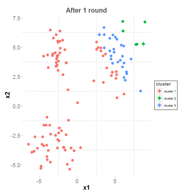
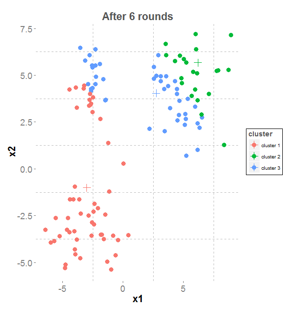
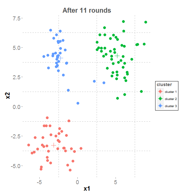
On the left side, the data points we want to cluster (generated by 3 gaussians). On the right side the clustering objective
Results of K-means iterations
Limitations The problem of K-means is that in can only discovered circles. If the datasets are to ovals, it may lead to unwanted results.
K-means can also lead to very unbalanced clusters, one clustering can contains 10% of data data, while another can contains 70% of the data.
Other clustering algorithms :
Expectation-Maximisation (EM) algorithm
Hierarchical clustering. For instance let's start with n points, glue together the two closest points. Compute their mean to be a new data point. Iterate until you meet the top.
Clara (Clustering LARge Applications)
...
Discovering latent factor
The other name of discovering latent factor is dimensionality reduction. When working with high dimensional data (thousands of variables per observation) one may want to reduce a much more smaller number
of variable understandable by a human. The goal can be obtain by different projections techniques of the points on space of smaller dimension. Moreover, we may have thousands of variables but the degree
of freedom may be much smaller corresponding to the latent factor we want to discover.
The most common dimensionality reduction technique is PCA (Principal Component Analysis) where the solution resides in selecting the most important direction. For instance, if the points form a very wide
ellipse, we can keep the projection of the points on the wide direction as a lower dimensional representation of the points.
Matrix completion
Matrix completion occurs when data are missing in the original datasets and we want to fill out the blank. For instance, there can be missing values from a survey that we want to fill. This could be solved
by supervised learning by predicting each column at a time using only line where there are no missing values, but if the problem is sparse (many missing values), supervised learning won't be of any help. Others
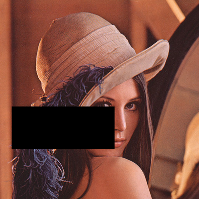
exciting applications are image inpainting (there is a shaded area on our image, and we want to know what was originally on the picture) or recommender systems (users have seen/like some products/movies and we
want to fill out the blank, i.e now their feelings, about unseen items). Recommender systems are known to be very sparse problem, often 97% of values are missing and the aim is to fill the ratings matrix composed
of n lines (one for each user), p columns (one for each product) and each entry is the rate of the given user for the given product. Such problems had been strongly studied for the netflix challenge.
Inpainting on Lena image. A frequently used image in computer vision
Reinforcement Learning
Presentation
The main difference between reinforcement learning (RL) and (un)supervised learning is that RL is in direct interaction with the environment. In RL, we modelise an
agent that must choose an action at a given time step t in a function of the context. Then the agent observe the consequence of his action (called the reward) and
update his strategy given this reward for the next step. It can be summarise as a loop :
The agent perceives state $s_t$
The agent performs action $a_t$
The environment evolves to state $s_{t+1}$
The agent receives reward $r_t$
Markov Decision Processes
A Markov Chain is a sequence of action where the next state depends only on the previous state and not on everything that could happened before. Mathematically
it is written : $\mathbb{P}(x_{t+1}|x_t,x_{t-1},\cdots,x_1,x_0) = \mathbb{P}(x_{t+1}|x_t)$.
An example of a markov chain is a walking process to go from a point A to a point B, and you want to find the quickest way to reach B. From time to time, you check
your map to see if your walking in the right direction. The direction you should take to reach B only depends on where you are right now and not on where you've been before.
A Markov Decision is form of :
The space of state $X$. It is all the possible states the context the agent his living in can take
The action space $A$. It is all the possible actions the agent can performs at each time step
The transition probability $p(y|x,a)$. It models the probability of being in state $y$ if the agent performs the action $a$ in state $x$
The reward $r(x,a,y)$ which represents the outcome received when performing action $a$ while the state evolves from $x$ to $y$
Of course the reward and the transition probability are not known in advance, otherwise there would be no more prediction to make and we would just need
to perform the action (or succession of action) that will maximise the overall reward. I precise overall reward because the goal is not to get the maximum
reward at each time step but have the maximum sum of the reward. For instance, when going on holiday by car, the best strategy is not necessary to go straight
in the target direction like a bird, but make a small detour (that will lower the short term reward) in order to reach the highway (and thus maximise the long
term reward).
The aim is to find the policy $\pi$ that will tell us what action to perform in state $x$ at time $t$ in order to maximize the sum of the rewards.
So the action $a$ will be $\pi_t(x)$. Formally, the aim is to find the policy that will maximise the following quantity, called the value function :
$$V^{\pi}(x) = \mathbb{E}[\sum_{t=0}^{\infty} \gamma^t r(x_t,\pi(x_t))|x_0=x; \pi]$$
Let's stop a moment on this formula.
Why an expectation? The process if probabilistic, meaning that taking twice the same action in the same state won't necessary lead to the same next state.
So the estimation must be average on a huge amount of time action $a$ is taken in state $x$. That is what the expectation models
Why $\gamma$? Mathematically we need the infinite sum to exists meaning that it must be equal to something and not the infinity. To do so, we weight the reward
by a factor $\gamma$ between 0 and 1 (exclude). If $\gamma$ is close to 0, the value function will focus on short term rewards, if close to 1 on long term rewards
What is $x_0$? $x_0$ is the starting state that will condition all the strategy for the problem being studied. Going from Atlanta to Chicago is not the same problem
as going from New York to Chicago
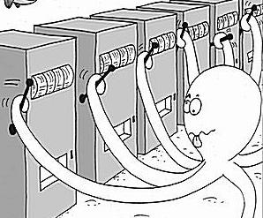
The Multi-arm Bandit Problem
Which slot machine pays most? Will you try each machine an equal number of times, sufficiently long and compare the average reward of each slot? The Multi-Arm Bandit (MAB) framework is dommed to
answer this question. More formally MAB help to tradeoff between exploration (try each different possibility in order to observe what happen) and exploitation (choose the best possibility as far
as we know). Of course you don't want to fully explore because after a while you know which possibility (called arm now) doesn't work so you stop testing it, but you can't also fully exploit because you must acquire
knowledge to know which arm is the best. Moreover, in some applications, new arms keeps coming, like for news article recommendations, new article are coming every day so you must explore
the performance of this new articles otherwise you will never recommend new articles.
The two mosts know MAB algorithm are :
$\epsilon$-greedy : $\epsilon$ per cent of the time, choose an arm at random and observe what happens. The rest of the time, choose the best action observed so far. The higher $\epsilon$
the more you explore. This strategy is obviously not optimal in most cases but answer the issue. Indeed, you keep testing from time to time new arm or previously suboptimal arm. You want to
keep testing suboptimal arm because maybe the few times you test it you were unlucky, so you want to be sure it is really suboptimal.
Upper Confidence Bound (UCB) : The UCB strategy performs exploration and exploitation in the same time ! The idea is to first compute the average performance for each arm, and instead of pulling
the best arm like you would do if you were exploiting, you then compute a confidence interval around the average performance. The upper bound of this confidence interval is function of the number of
times you pull this particular arm and the number of time you pull an arm. Indeed, the most often you pull an arm, the most confidence you are about what is the performance of this arm. Let's suppose
you pull the arm $j$ $n_j$ times and you pull an arm $n$ times. Moreover, let's note $r_j^n$ the average reward of arm $j$ after $n$ trials. The upper bound is compute as follow :
$$ub_j^n = r_j^n +\sqrt{\frac{ 3 \log n}{n_j}}$$
This bound increases with $n$ and drecreases with $n_j$. It increases with $n$ slower than it decreases with $n_j$ because otherwise the bound will keep increasing except if you pull the same arm over and
over. Thus, applying this formula, you get a box around the mean which is wide the first time you pull this arm, and decreases over time.
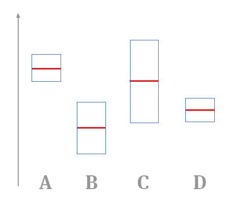
Still, we haven't answer the question of which arm should I pull? Let's imagine that we have 4 arms, and the corresponding graph where each red line correspond to average (expected) reward for each arm, and
the blue box represent the confidence bound around it. What arm would you pull? (The wrong answer is A ...)
The UCB tells you to choose arm C, because he is the one with the higher upper confidence bound. The idea is that in best case scenario it is the one that will perform the best. If it not the best, at least
choosing this arm will reduce its uncertainty because we will gain knowledge for this arm. In both case we are winning something. The catchphrase of UCB is "Optimism in Face Of Uncertainty", meaning exactly
the same : when facing uncertainty we choose the optimistic performance of the available arms. Of couse, if the upper bound of arm A were above the C one, we would pick A. We doesn't pick C because its uncertainty
is wide but because it is the highest.
There are many other algorithms are extension that uses context for instance, but I won't develop it here.
Conclusion
So by now you should know a lot about what kind of problems a data scientist can answer and what are his tools. What you don't know is how to compute the solution to all those problems. If you want to do so, the first
step would be to learn programming. Then you could just use package that solves those different problems but I'm not a big fan of that. I think it is important to understand what is behind the scene to understand why
it works, why it doesn't and how to improve the results. So you should learn more theoritical lecture about the solution of the problems, what are the caution to take and then you could use all those package ;)
Preprocessing data
From big data to smart data
Preprocessing data is mostly done by SQL(-like) request. As I am not writing a tutorial about SQL, this part will be shorter than the previous, however it is the most important part and the longest part in a data scientist day.
During the whole first part, we assume that a dataset with as many lines as example and as many columns as variables were available, and all what left to do is train a model. In real life, the data scientist has to
construct this dataset. In web application, what is available is a huge table with billions of lines where each line is a description of what the user did. This table has no order, and contains no variable at first. An extract of
such a table can look like this :
So we have a table with billions of lines with a line for each action/view of a user and we want a table understandable by our machine learning algorithm with a line per user or per session with
variables describing the user behaviour in columns. So for instance what we would like to have is the number of product clicked by the user, so you need a request understandable by the computer that
will compute this value for each user. You may want to know how many times he/she bought something, what was the average price, ... Those are variables quite easy to compute because those informations
exist in one line. But sometimes, you may want to know from which list of product comes the product the user just click. As you can see in the extract, the user is either on a list page and so we know the
list of product available on the page, or the user is on a product page and we know what this product is, but both informations are not available in the same lines. Moreover there is no order in the table,
so you cannot say to the compute "go get the previous line", and even if you could, maybe the previous line was a line from an other user ... So what you need to do his look in all the list of the same
user, check if the product you looking for is in, then compare the timestamp (time in seconds from the 1st january 1970), and find the closest timestamp in the past. You have to create such a request
that will do it for all product views and for all user in the same time. So not only some variables are complex to get, errors occurs, the request takes times, etc, but you also have to imagine all the
variable that could have an impact in your problem. Some are obvious other more original. So it is a back and forth movement between your machine learning algorithm and your huge input table in order to add and
drop variables and see which are relevant and which are not. This work can take 70% of the time ... and it is the most important work because a good algorithm is nothing without the right variables. Even
with the best algorithm of all time, you won't predict the weather from the number of chair in the room.
From smart data to input table
That is not the end ... You may have variables that are text, so variables cannot be treated by the algorithm. For instance you may have a variable "categorie" that take the values 'A', 'B', 'C'. The
solution is to create what are called 'dummy variable'. You create 3 variables categorie_A, categorie_B and categorie_C that take the value 1 if the categorie is the right one, 0 otherwise. To be
completly exact, you only (and must) create 2. Because the third depends and the two first : if you have 0 and 0 then third is 1, O and 1 then 0 and finally 1 and 0 then 0.
The last thing to do is ALWAYS CENTERED DATA. For now the variables can take any values, some are binary, some are a rate so between 0 and 1, some are continuous (price, time spend, ...). All those
variables are not comparable from one to another, so you need to transform the variables. There are mainly two possibilities :
Divide all the variable by their max value, thus all variables will be between -1 and 1 (between 0 and 1 if positive)
Substract the mean and divide by the standard deviation, thus all variable will spread around 0 depending on their standard deviation
It is now time to run the machine learning algorithm and be careful of the relevance of the variables.